
How To Measure Marginal Willingness To Pay via Conjoint Analysis (Pricing Research Guide)
Marginal Willingness To Pay measures how much a customer would spend to change one specific feature of your product.
Marginal Willingness To Pay is popular in customer research because it brings objective data to high-stakes pricing discussions that are often driven by opinions and emotions. It is considered an essential analysis format that every product builder, revenue leader, and UX research manager should have in their toolkit of methodologies.
Running a Marginal Willingness To Pay study is a lot easier than you would expect. Once you’ve read this guide, you’ll have everything you need to know— from the underlying theory to real examples and a step-by-step approach for running your own willingness-to-pay study.
Sections:
What Is Marginal Willingness To Pay?
Let’s start by breaking this down into two parts…
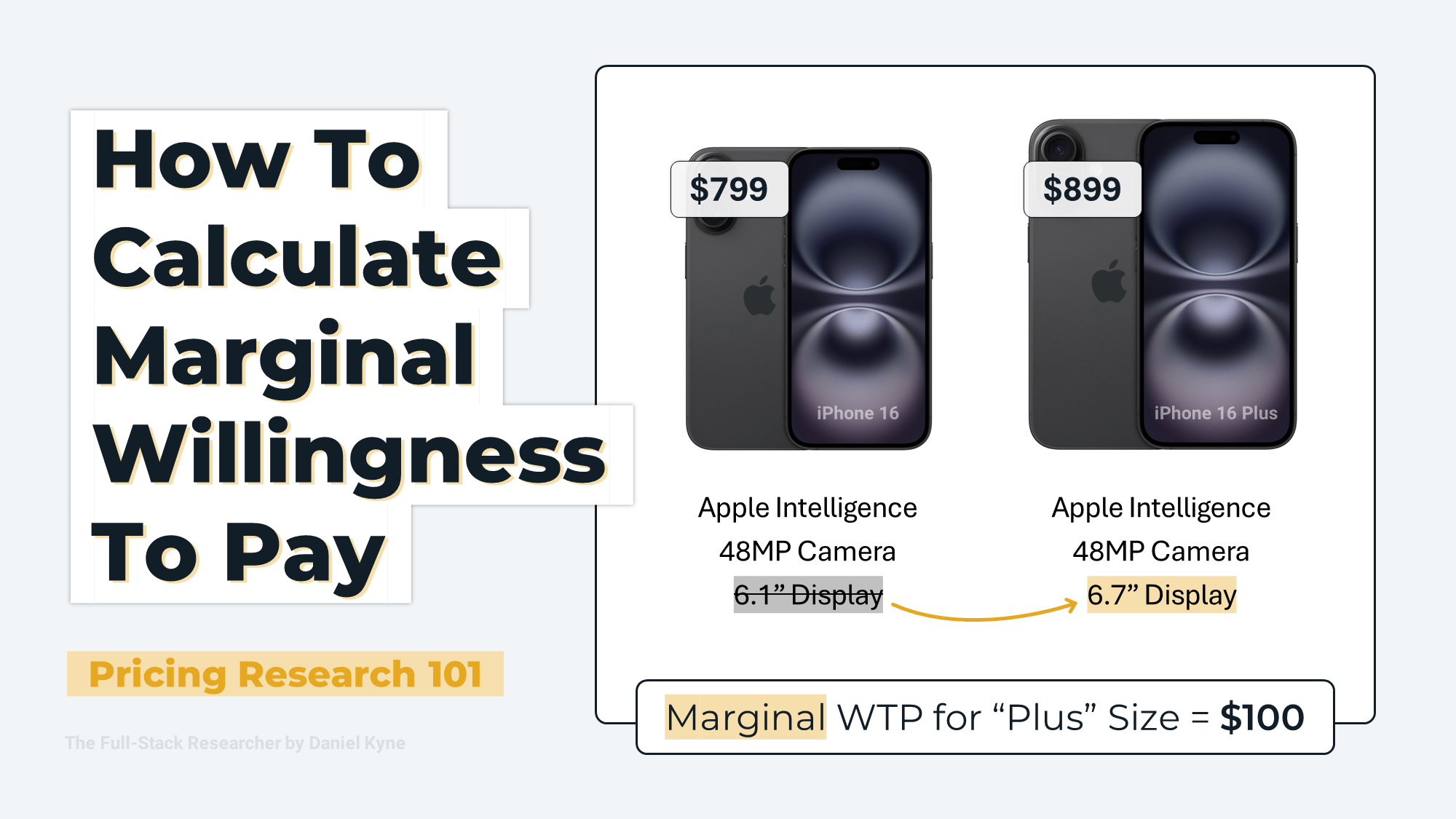
Willingness To Pay refers to how much money a customer would spend to purchase your product or service. For example, let’s say the average customer’s willingness to pay for the latest iPhone is $799.
Marginal Willingness To Pay tells us how much extra that same customer would pay to buy an iPhone 16 Plus instead of the default version with a 6.1” screen size. The word marginal here means “extra” or “incremental” — when compared to the baseline version, how much more or less does a customer value the product if you change just one of its characteristics.

If the average customer’s WTP for a standard iPhone 16 is $799 and they would pay $899 for the iPhone 16 Plus with a larger screen but otherwise same specs, then we could say that the Marginal Willingness To Pay for the larger screen is $100. In this example, MWTP is not the overall value of the product or the value of a 6.7” screen in isolation, we’re comparing how much more or less someone would pay for this specific upgraded version compared to the baseline model.
What can you use a Marginal Willingness To Pay study for?
Understanding how customers value different aspects of your product in a measurable way is extremely useful in many scenarios — here are just a few examples of how you could use this data:
Optimizing Monetization: See whether you’re undervaluing pricing tiers by looking at how much customers would pay for each of the upgrades you’re offering on premium tiers compared to your base plan.
Premium Marketing: Identify which features on your premium plans have the highest marginal willingness to pay and focus your product marketing efforts on making these the “headliner” features promoted to potential customers.
Expansion Opportunities: Instead of just looking at the MWTP within your overall customer base, you can segment your results to find groups that value particular features significantly higher than the average user, helping you identify features that could be spun out into optional paid add-ons.
Prioritizing High-Value Features: Running a MWTP study with unreleased features is a great way to understand which hypothetical product additions are considered the highest value to customers.
What Data Is Required To Calculate Marginal Willingness To Pay
Marginal Willingness To Pay is calculated using the results of a survey format called conjoint analysis. This entire guide is based on analyzing the results of a conjoint analysis survey. Don’t let this deter you — conjoint surveys are easy to run and there are free tools that offer conjoint surveys with unlimited participants.
What is Conjoint Analysis?
Conjoint analysis is a survey format where people are shown a series of products, each with different features and prices, and asked to vote for the one they prefer most. Their choices reveal which product attributes are most important to them and the most preferred version of each feature. Here’s what it looks like to vote on a conjoint survey:
^ In this example, you can see the brand attribute has many options like iPhone, Google Pixel, and Samsung.
For example, imagine you’re planning a family BBQ on a small budget and you’re trying to decide which burger ingredients to buy. You can’t afford to buy multiple of every option, so you run a conjoint analysis survey to see which attributes are most important to people (patty, sauce, salad, bun) as well as which options are most preferred for each attribute (like chicken, beef, or vegan for the patty attribute).

^ These results show us that the Patty attribute has the widest range in scores and therefore is the attribute that affects people’s choices the most, while the Sauces have a much narrower range of scores. I can use this info to prioritize buying more patty types and spending less of my budget on buying many sauce types.
Conjoint analysis is an ideal research method to use in cases with non-fungible attributes — many separate parts of a decision that can’t be excluded, like how you can’t exclude the buns while still calling it a burger! If you’re trying to model how people make a decision that has two layers of information (categories and options within each attribute), then conjoint analysis is a great way to do that. If you want to take a moment to dive deeper into conjoint surveys, I’d recommend taking a look at my ultimate guide to conjoint analysis.
Conjoint Analysis for Pricing Research
This is why conjoint analysis is so commonly used in pricing research, especially for tech companies — just like the burger example, a pricing plan is made up of a list of attributes (price, seats, credits, integrations, feature capabilities, etc.) and each attribute has many potential options. Conjoint analysis tells a team which of these attributes influences customers’ decisions most and which configuration of options would drive the most overall demand or revenue.
So now we know what goes into a conjoint analysis survey; attributes and options. What does the output of a conjoint analysis study look like?
If you use a research tool that has a conjoint analysis survey format (like OpinionX, which offers it for free with unlimited participants per survey), then the research tool will automatically turn people’s votes into a “utility score” that represents each option’s relative importance. Here’s an example of what conjoint results look like as a data table and a preference chart:
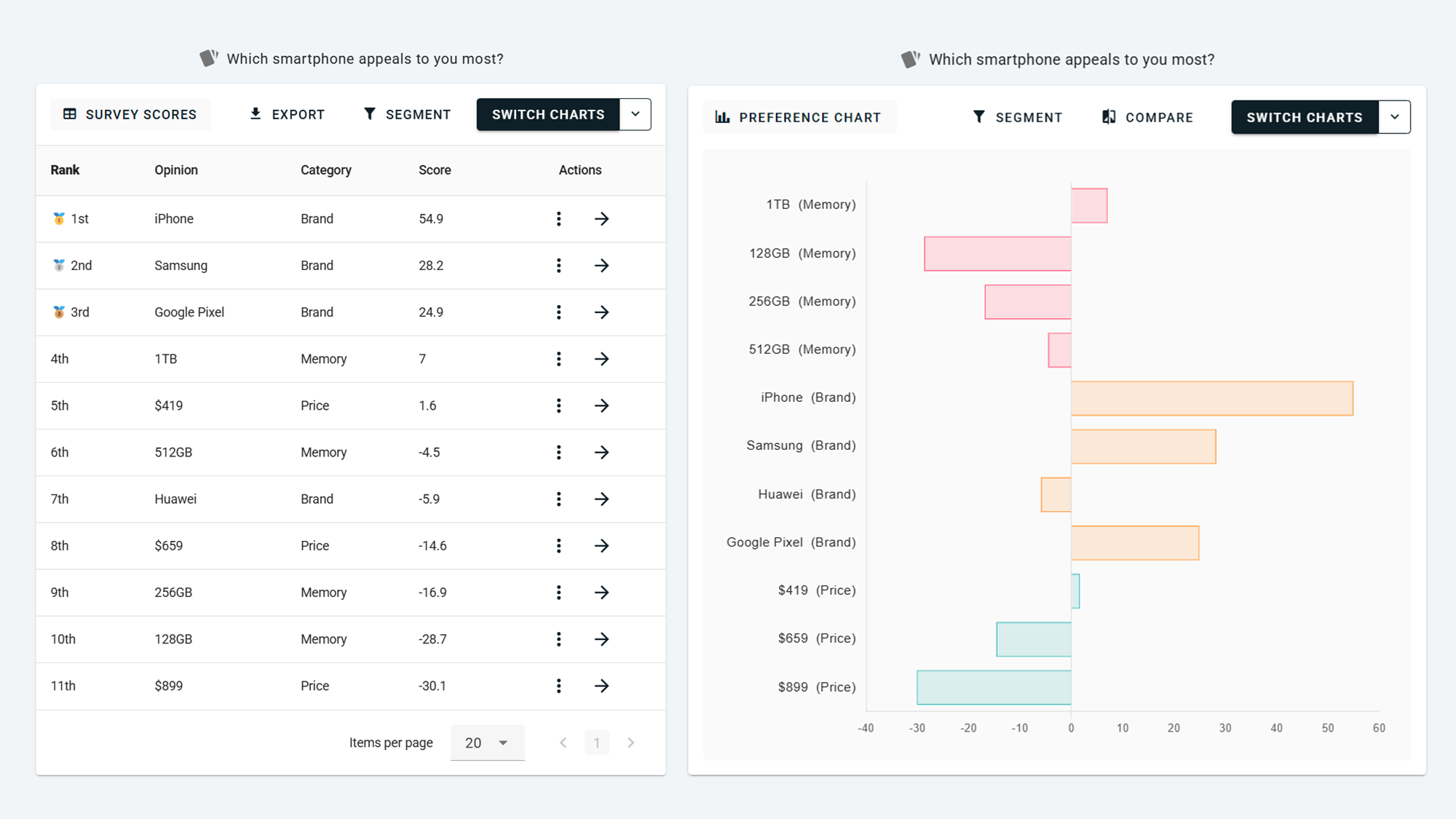
These scores from a conjoint analysis survey show an option’s relative importance — the numbers alone don’t tell us how much people love or hate something in isolation, they only show us how much more or less they prefer one option over another.
However, we can use a simple method to turn these relative scores into relative financial value in actual dollar terms. By looking at the utility scores for different prices, we can see how much a change in price causes a change in score to calculate how much each point is worth in dollars.
To explain further, take a look at this simple conjoint results table:

Increasing the price from $100 to $200 caused the score to decrease by 20 points. $100 divided by 20 points means every $5 price increase led to a change in score of 1 point. We can use this to assume that customers value each point of utility at $5 for the other attributes in our conjoint survey.
Looking at the Color attribute, we can see that there is a 12-point gap between sizes Gray and Gold. By multiplying 12 points by $5 per point, we could say that customers value the Gold product $60 more than the Gray version, in relative terms. This doesn’t mean they would definitely pay $60 more to upgrade from the small to the large product, but that the perceived value difference is equivalent to a $60 price change.
There are a couple of things you should take from this example:
To conduct MWTP analysis, your conjoint survey needs a “price” attribute with 2 or more options.
MWTP results tell us the relative financial worth of one option compared to a baseline option (eg. Gold vs Gray). It doesn’t tell us a total willingness to pay, just the relative difference.
This is not so complicated really! Even non-professional researchers can run studies like this :)
Let’s jump into the details and see how to create a Marginal Willingness To Pay report from a more realistic user research project using conjoint survey…
How To Calculate Marginal Willingness To Pay from Conjoint Analysis
I’ll show you how to create a MWTP report in two ways:
Generated automatically on a research tool like OpinionX.
Created manually from raw conjoint data on Google Sheets.
The example I’ll be using throughout this guide is from the same smartphone preferences survey that was shown in a GIF at the start of this guide:

Option 1: Automatic MWTP Report via OpinionX
OpinionX is a modern market research tool that offers free conjoint analysis surveys with unlimited participants per survey. Your conjoint results on OpinionX will be displayed as a data table like in the screenshot below, where you can see the utility scores that represent the relative importance of each option according to survey respondents.

Next we need to understand the relationship between price and score. OpinionX gives you a graph with price on the x-axis and utility score on the y-axis. The three gold dots on the graph below are our three price points ($419, $569, $899) and a trendline is plotted between the three of them:

This trendline shows us the relationship between price and score, ie the price per utility. This is all done for us automatically so we don’t need to worry about calculating it manually, but you can always see the underlying data — the trendline equation and the R² (how well the trendline fits your data) — by clicking the “Configure” button:

Below the price/utility chart, you’ll see the marginal willingness to pay for each option. There will be one blank row per attribute group — this is the baseline option that you’re comparing the other options against. Click any bar on this chart to turn that option into the new baseline comparison option, or choose all your baseline options from the Configure menu. These results show us that customers value an upgrade from 128GB of smartphone storage to 256GB as being worth $162.34, in relative terms.

The best part about doing this analysis using an automated tool is that you can filter the results to see how they change if you only include a certain type of customer. For example, by clicking the “Android” bar on the bar chart below this, I activated a filter to exclude everyone except current Android customers. We can see that the MWTP report changes a lot now, with the relative value of iPhone as a brand dropping considerably:

Try it for yourself! You can access the interactive results of this survey here without any login or sign-up required. To find the MWTP report, just scroll down to the conjoint analysis results table, click the “Switch Charts” button, and choose the Willingness To Pay format:

Personally, the value of segmenting your MWTP results can’t be stressed enough. The goal here isn’t just to find how much customers value specific features, but to find which customers value upgrades the most. You can only accomplish this via segmentation analysis on an automated MWTP chart like the one on OpinionX, which is not possible using the manual method explained below.
Option 2: Manual MWTP Report via Google Sheets
There are four steps required to turn conjoint survey results into a Marginal Willingness To Pay report:
Utility Scores
Marginal Utility
Dollars Per Utility
Marginal Willingness To Pay
At the end of these four steps, you’ll have a Marginal Willingness To Pay report that looks like this:

Starting with a blank spreadsheet, I’ll create a simple table with my categories, options, and four columns for each of the four steps we’re about to do:

Step 1: Utility Scores
Copy the utility scores for each option from your conjoint analysis survey and paste them into your spreadsheet. These utility scores are shown for free on your OpinionX survey results, even if you’re not on a premium pricing plan.

Step 2: Marginal Utility
Marginal Utility is the difference in score between two options. This step has two parts:
Baseline Version → what product configuration are we comparing other versions against?
Marginal Scores → difference between the baseline and alternative options in each category?
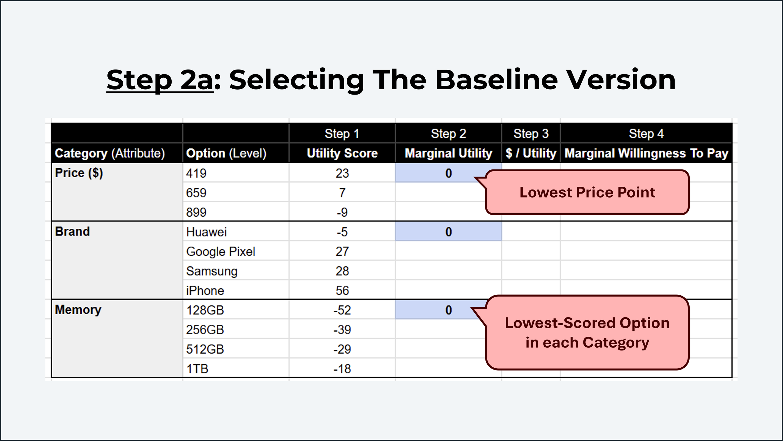
To start, let’s select our baseline version. I usually keep this quite simple by picking (i) the lowest price point and (ii) the lowest-scored option from each category. For each of these, I give it a “Marginal Utility” score of 0, which we’ll use as our comparison benchmark for other options:
Next we calculate Marginal Utility by taking each option’s score and subtracting from it the baseline score from the same category. Here’s how that looks for just the Brand category:

Once finished, you’ll have a completed table like the one below. These “Marginal Utility” numbers tell us how much more/less someone values an option compared to the baseline option — for example, people value Google Pixel phones “32 points” more than Huawei phones. But what are these 32 points worth in dollar terms? That’s what we’ll figure out next…

Step 3: Dollars per Utility
To figure out how much extra these “marginal utility” numbers are worth in financial terms, we’ll calculate the relationship between how much the price changed and how much the points changed. To do that, we’ll use the formula (Price2–Price1)/(Utility2–Utility1). You can see this formula in action in the screenshot below:

In this case, we have a linear relationship between price and utility — ie. for all price point gaps, a decrease in price of $15 is equal in value to 1 utility point. In some cases this relationship is not linear, but I will explain later in this guide how to identify and deal with such scenarios. At the end of this guide, I offer some specific suggestions about how to deal with non-linear price/utility relationships.

Step 4: Marginal Willingness To Pay
The formula for Marginal Willingness To Pay is -MU*DPU, where MU means “Marginal Utility” (the number we calculated in step 2) and DPU means “Dollars Per Utility” (the number we calculated in step 3). In the example above, you can see this formula in action on our spreadsheet. It’s actually quite simple — just remember to include the minus sign!
How To Create a Marginal Willingness To Pay Graph
There are two main components shown in the example of the MWTP report above:
Marginal Willingness To Pay Chart that shows how much a customer would pay to switch between the baseline version of the product versus a specific upgrade to one attribute.
Price/Utility Graph visually shows the relationship between price points and their respective utility scores, which forms the basis for the financial analysis in our MWTP chart.
Both of these report components can be created on Google Sheets using the manual method outlined in this guide or you can use the premade automated template that comes with conjoint analysis surveys on OpinionX.

What should you do when price and utility create a non-linear pricing curve?
In most cases, the relationship between price and utility is not perfectly linear. This means that price increases affect the utility score in different ways depending on whether the change is at the higher or lower end of your prices.

Here’s how a linear price/utility relationship looks.
You can see that every dollar change in price causes a consistent change in score, regardless of whether it happens at the low or high end of the price range.
Not all price/utility relationships are like this — in fact, it is uncommon for this to be the case! Most of the time, price/utility will look more (1) Curved, (2) S-Shaped, or (3) U-Shaped.
Let’s look at each in more detail…

1. Curved Line:
In the example above, customers care a lot more about small price increases when the price is low (between $30 and $50, even a minor price increase impacts utility significantly). However, as prices increase beyond $50, the sensitivity decreases. Each additional dollar added above a price of $70 has less of an impact on utility compared to each dollar increase between $30-$50. The curve helps identify price points where consumers are most and least sensitive, which can be critical for pricing strategy.

2. S-Shaped
In the example S-Shaped curve above, the highest price sensitivity is found near the middle of the price range around $30-$80 (the section with the steepest slope). Price sensitivity reduces dramatically above $100+ (seen in the “flattening” of the curve), meaning that the impact that price increases at this range have on customer preference reduces with each additional dollar added.

3. U-Shaped
In this final example, the price/utility relationship is almost linear until the sharp change between $150-$200, creating a U-Shaped curve. Numerous factors that could explain this… It could be the “perceived quality” effect, where some customers associate a higher price with a potential improvement in quality, brand prestige, or exclusivity. Alternatively, it could be an “anchoring effect”, where the customer associates the product’s quality with a known competitor that also uses a $200 price point. Or it could be an “even number” bias, where people are more likely to associate quality with a price that contains more zeros instead of other digits (we humans are simple creatures really).
So how do you create a MWTP report when Price/Utility is non-linear?
Non-Linear Price/Utility Curves are a problem when it comes to manually calculating a Marginal Willingness To Pay report because the Dollars Per Utility metric fluctuates between price points. Here’s how I would approach this.
A. Trendline Analysis
Both the Curved Line and S-Shaped examples were almost linear — the curves stay close to their trendlines. We can use a calculation called R² (“r squared”), more officially known as “the coefficient of determination,” to see how well the trendline fits the curve it is based on.
When R² = 1, that means the trendline and curve perfectly match. An R² above 0.95 is an “Excellent Fit” and can be used as a linear replacement for our curved Price/Utility chart. An R² between 0.95-0.90 is an “Acceptable Fit” and can cautiously be used depending on the shape of the curve. An R² of 0.90-0.85 is a “Questionable Fit” that should not be used in most cases, and anything below 0.85 is an “Unsuitable Fit” which definitely should not be used.

The easiest way to do this is using Google Sheets, which will automatically give you the trendline, the equation for the trendline, and the R². Here’s exactly how to do that:
Create a simple table with price points and their utility scores.
Turn this into a line chart.
Go to Chart Editor → Customize → Series, and do the following actions:
a. Enable “Trend line”.
b. Change the “Label” dropdown to “Use equation”.
c. Enable “Show R²”.
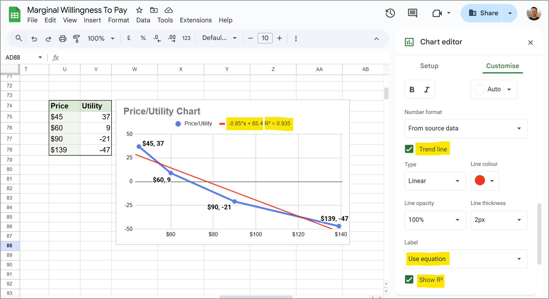
You can then see the two key outputs you’re looking for highlighted on the chart above — the trendline equation and the R² result. In this case, our R² is 0.935, which falls into our Acceptable Range (not ideal, but usable).
Next, let’s turn this trendline equation into our dollars per utility metric that is required for the rest of the MWTP analysis.
In the example above, my trendline equation is y=-0.85x+65.4. Dollars Per Utility basically means “how much of a change in price on the x-axis causes ±1 for the score on the y-axis.” Figuring this out is actually quite easy — just divide 1 by whatever comes before x in the equation (in this case, -0.85).

So 1/-0.85 equals -1.17647, which means that for roughly every $1.18 added to the price, the utility score goes down by 1 point. This is the number we will use as the financial input when calculating Marginal Willingness To Pay for our conjoint survey’s various options.
B. Exclude Outlier Price Points
The U-Shaped price/utility curve shown here has an R² of 0.846, which falls into the Unsuitable Fit definition. While this trendline should not be used, it’s clear that the poor fit is being caused by the $200 price point.
While this is definitely something that should be investigated further by the researcher (potentially caused by prestige effect or a market anchor from a competitor product), for the purposes of your MWTP analysis, you could consider excluding this price point from your analysis. This is possible to do in just one click on OpinionX (on the Configure Tab, just hit the “x” icon beside the $200 price to exclude it from the automated MWTP report.
Getting your first Marginal Willingness To Pay study started…
The first step of any MWTP study is to create your conjoint survey.
To learn more about conjoint analysis in UX research, check out my ultimate guide to conjoint analysis.
If you’re ready to get started, I recommend checking out OpinionX which has a free tier that includes unlimited conjoint analysis surveys with unlimited participants per survey too.
— — —
Enjoyed this blog post? Tens of thousands of founders and product teams subscribe to our newsletter, The Full-Stack Researcher, for actionable user research advice like this guide delivered straight to their inbox:
About The Author:
Daniel Kyne is the Founder & CEO of OpinionX, a market research tool for modern product teams — used by thousands of researchers to better understand what matters most to their customers. OpinionX is a leading platform for conjoint analysis and comes with an easy-to-use Marginal Willingness To Pay report. Create a free Conjoint Analysis survey on OpinionX today!